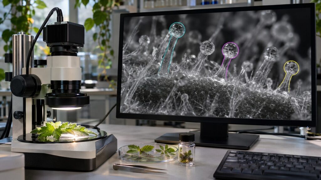
The easiest gland to count is the one standing by itself, sharply in focus against an empty background. Then comes the pair with overlapping heads. Then the one cut in half by the edge of the picture. By the time a botanist reaches the end of a microscope image, “count the glands” has turned into a surprisingly long set of decisions. Teaching a computer to do it means making those decisions visible.
What earns a mark on the image?
The glands are trichomes, small outgrowths on the surface of a plant. On cannabis flowers, some contain specialized secretory cells and have a rounded head. A person marking a photograph can draw a boundary around each visible head or place a point at its center. Those two exercises create different data. A point can support a count. A boundary can also give an estimate of size, provided the image has a scale and the outline is accurate.
In research combining deep learning with the study of cannabis trichomes, automated measurement helped investigators examine how gland formation varied under the conditions they studied. The attraction is straightforward. Once a counting method works, investigators can examine many more views with a consistent set of rules. But a computer can be remarkably consistent about making the same mistake on every photograph.
Ten counted, two missed
Suppose a human examiner marks ten glands. A program also reports ten. That sounds like perfect agreement until someone overlays the marks. Perhaps the program missed two small glands and counted two bright reflections instead. The total happened to come out right. Checking which marks coincide tells the investigator something the grand total cannot.
Scientists distinguish errors of omission from false detections. A tool that overlooks small objects may introduce a bias into comparisons between younger and older flowers. A tool that splits bright heads in two may manufacture a difference between images taken under different lighting. Both problems can survive a test that looks only at average counts. An error map, with individual mismatches marked where they occur, gives the person at the microscope somewhere to look.
A new photograph can be too familiar
When examples from the same microscopic field appear in both the material used to build a model and the material used to evaluate it, a high score may overstate what the model has learned. Nearby image patches can share an unusual shadow or the exact outline of a damaged gland. A more demanding trial asks the method to work on a different specimen, and ultimately on images taken under conditions it has not encountered before.
The biology makes that challenge more than a technical nicety. Microscopy across stages of flower maturation documented changes in gland form and autofluorescence. If a program learns that a certain bright shape identifies a gland, what will it do with the same kind of structure at an earlier stage? Looking carefully at mistakes can reveal that the biological category itself needed a more careful definition.
Counting glands and counting plants
A final distinction matters after every detection has been checked. Ten thousand glands photographed on two plants provide detailed information about those two plants. They are still only two independent plants. Treating each detected gland as an independent replicate can make a biological conclusion look more precise than the sampling design allows. A sound analysis keeps the link from gland to image to plant intact. Work on how to average cells in microscopy experiments illustrates why taking more images and adding independent specimens solve different problems.
Automation earns its place when the time saved at the microscope can go into better sampling and better checks. The most persuasive result is rarely a single impressive accuracy figure. It is a collection of images in which you can see the objects counted correctly, the awkward cases and the conditions under which the method starts to fail. A botanist who knows where the computer loses count can put the next hour of human attention exactly there.